Simulation Function

library(ggplot2)

## Warning: package 'ggplot2' was built under R version 3.4.4

CHIANOVA <- function(ngroups = 5, pergroup = 12, plot = F){
  intDat <- round(runif((ngroups*pergroup),1,100))
  catDat <- factor(rep(1:ngroups,(60/5)))
  
  df <- data.frame(intDat,catDat)
  t <- xtabs(~intDat + catDat, data = df)
  ch <- chisq.test(t)
  
  m <- aov(intDat ~ catDat, data = df)
  sm <- summary(m)
    if (plot){
    print(ggplot(df, aes(x = catDat, y = intDat)) + geom_boxplot(aes(fill = catDat)) + theme_classic())
  }
  return(list(chi = ch$p.value, anov = sm[[1]][["Pr(>F)"]][1]))
}

Example of Simulation Run

examp <- CHIANOVA(plot = T)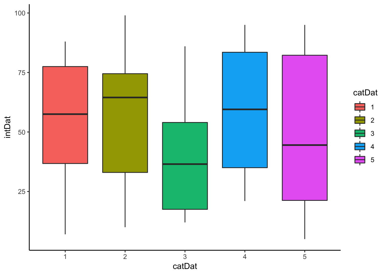

## Running the Simulation

set.seed(123)
n <- 1000
ca <- data.frame(chi = 0, anov = 0)
for (i in 1:n){
  k <- CHIANOVA()
  ca <- rbind(ca,k)
}

ca <- ca[2:dim(ca)[1],]
head(ca)

##         chi       anov
## 2 0.2752663 0.94383179
## 3 0.5824732 0.35307383
## 4 0.5427126 0.54559270
## 5 0.1378418 0.68759501
## 6 0.6919098 0.09748467
## 7 0.4859818 0.50135175

Plots

ggplot(ca,aes(x = chi, y = anov)) + geom_point() + geom_smooth(method = "lm")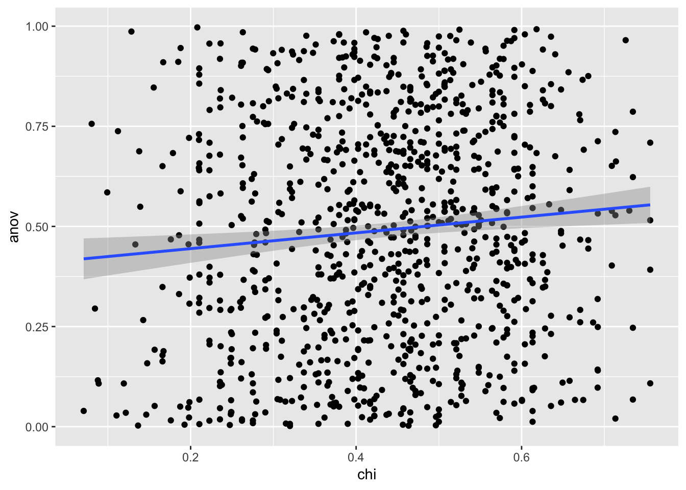

cor(ca)

##             chi       anov
## chi  1.00000000 0.09304987
## anov 0.09304987 1.00000000

chi_aov <- lm(anov~chi, data = ca)
summary(chi_aov)

## 
## Call:
## lm(formula = anov ~ chi, data = ca)
## 
## Residuals:
##      Min       1Q   Median       3Q      Max 
## -0.52535 -0.24430  0.00169  0.23500  0.55619 
## 
## Coefficients:
##             Estimate Std. Error t value Pr(>|t|)    
## (Intercept)  0.40517    0.03042  13.319  < 2e-16 ***
## chi          0.19682    0.06666   2.952  0.00323 ** 
## ---
## Signif. codes:  0 '***' 0.001 '**' 0.01 '*' 0.05 '.' 0.1 ' ' 1
## 
## Residual standard error: 0.2829 on 998 degrees of freedom
## Multiple R-squared:  0.008658,   Adjusted R-squared:  0.007665 
## F-statistic: 8.716 on 1 and 998 DF,  p-value: 0.003227

Density Plots of p-values

#distribution of p-values density, makes sense that the p-values for anova are skewed because there's a clear effect.
ggplot(ca,aes(x = chi)) + geom_density()

ggplot(ca,aes(x = anov)) + geom_density()

ggplot(ca) + geom_density(aes(x = chi)) + geom_density(aes(x = anov))

The density plot of the anova p-values is relatively flat, which is expected given a null effect. The density plot for the chi-square p-values is not flat, with a peak around 0.5. ## What did we learn?

In our simulation, there is a small positive correlation between the p-values you get when you run an ANOVA and chi-square test on data that has a continuous but integer outcome, and a categorical predictor when the null is TRUE.

However, the adjusted \(R^2\) value is incredibly low at ~ 0.009, indicating that knowing the p-value of the chi-square test on the data does not explain much of the variation in the p-value of the ANOVA test on the same data.

In layman’s terms, there’s not a strong relationship between the p-values you get with the two different tests. This makes sense since when you run a chi-square test, you treat your continuous/integer value as a categorical variable. Which is is not.

Simulation Function

CHIANOVA2 <- function(ngroups = 5, pergroup = 12, plot = F){
  intDat <- round(runif((ngroups*pergroup),1,100))
  catDat <- factor(rep(1:ngroups,(60/5)))

  
  df <- data.frame(intDat,catDat)
  
  #creating a relationship
  df[df$catDat == 1, "intDat"] <- df[df$catDat == 1,"intDat"] -5
  df[df$catDat == 2,"intDat"] <- df[df$catDat == 2,"intDat"] -25
  df[df$catDat == 3,"intDat"] <- df[df$catDat == 3,"intDat"] + 20 
  df[df$catDat == 4,"intDat"] <- df[df$catDat == 4,"intDat"] + 2
  
  t <- xtabs(~intDat + catDat, data = df)
  ch <- chisq.test(t)
  
  m <- aov(intDat ~ catDat, data = df)
  sm <- summary(m)
  if (plot){
    print(ggplot(df, aes(x = catDat, y = intDat)) + geom_boxplot(aes(fill = catDat)) + theme_classic())
  }
  return(list(chi = ch$p.value, anov = sm[[1]][["Pr(>F)"]][1]))
}

Example of Simulation Run

examp <- CHIANOVA2(plot = T)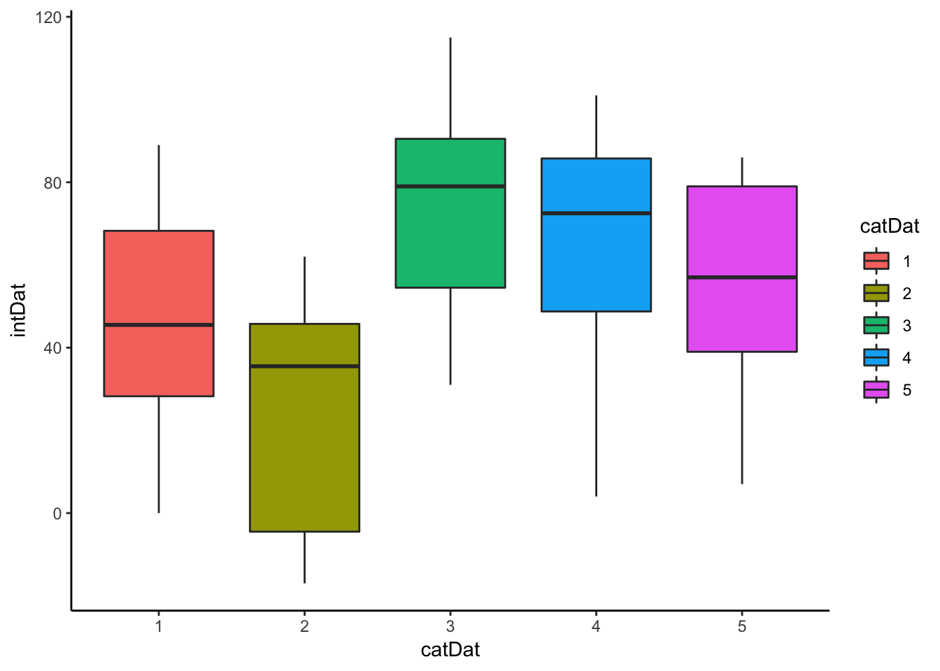

Running the Simulation

set.seed(123)
n <- 1000
ca <- data.frame(chi = 0, anov = 0)
for (i in 1:n){
  k <- CHIANOVA2()
  ca <- rbind(ca,k)
}

ca <- ca[2:dim(ca)[1],]
head(ca)

##         chi         anov
## 2 0.2337785 4.776362e-03
## 3 0.5912555 4.387574e-03
## 4 0.4899230 5.786586e-03
## 5 0.1987483 6.079448e-05
## 6 0.4671540 2.377428e-03
## 7 0.5736945 4.157098e-02

Plots

ggplot(ca,aes(x = chi, y = anov)) + geom_point() + geom_smooth(method = "lm")

cor(ca)

##             chi       anov
## chi  1.00000000 0.04989023
## anov 0.04989023 1.00000000

chi_aov <- lm(anov~chi, data = ca)
summary(chi_aov)

## 
## Call:
## lm(formula = anov ~ chi, data = ca)
## 
## Residuals:
##      Min       1Q   Median       3Q      Max 
## -0.03191 -0.02370 -0.01939 -0.00720  0.61377 
## 
## Coefficients:
##             Estimate Std. Error t value Pr(>|t|)  
## (Intercept) 0.014516   0.006365   2.281   0.0228 *
## chi         0.024775   0.015700   1.578   0.1149  
## ---
## Signif. codes:  0 '***' 0.001 '**' 0.01 '*' 0.05 '.' 0.1 ' ' 1
## 
## Residual standard error: 0.06304 on 998 degrees of freedom
## Multiple R-squared:  0.002489,   Adjusted R-squared:  0.00149 
## F-statistic:  2.49 on 1 and 998 DF,  p-value: 0.1149

#distribution of p-values density, makes sense that the p-values for anova are skewed because there's a clear effect.
ggplot(ca,aes(x = chi)) + geom_density()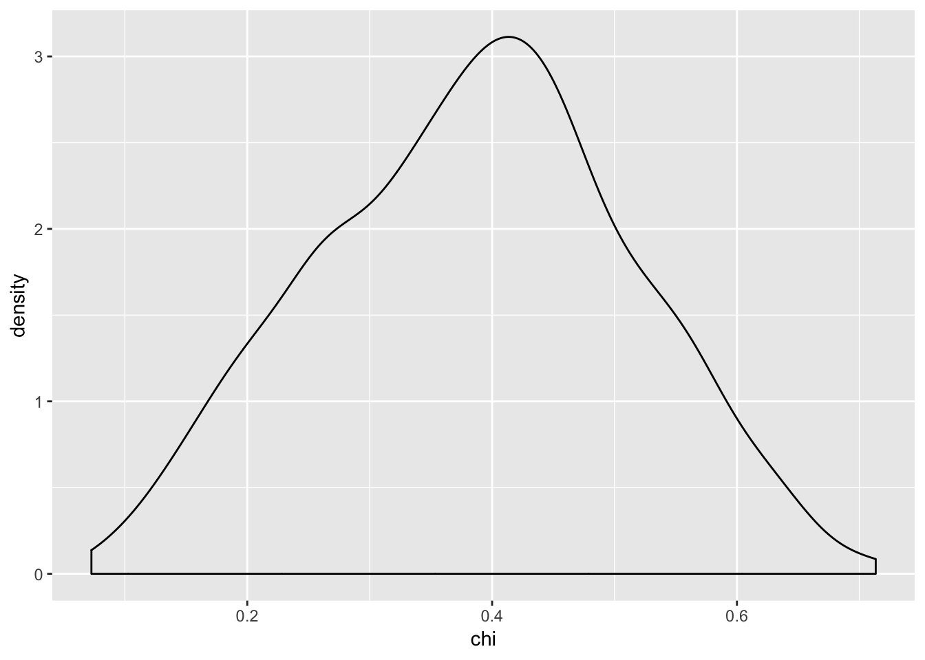

ggplot(ca,aes(x = anov)) + geom_density()

ggplot(ca) + geom_density(aes(x = chi)) + geom_density(aes(x = anov))

#distribution of p-values density, makes sense that the p-values for anova are skewed because there's a clear effect.
ggplot(ca,aes(x = chi)) + geom_density()

ggplot(ca,aes(x = anov)) + geom_density()

## What did we learn?

Again, there is a small positive correlation between the p-values you get when you run an ANOVA and chi-square test on data that has a continuous but integer outcome, and a categorical predictor when the null is FALSE.

We get a small adjusted \(R^2\) value here as well of ~ 0.002.

From our simulation here, it looks like regardless of the relationship between our two variables, running a chi-square test and an ANOVA will give you virtually unrelated p-values.